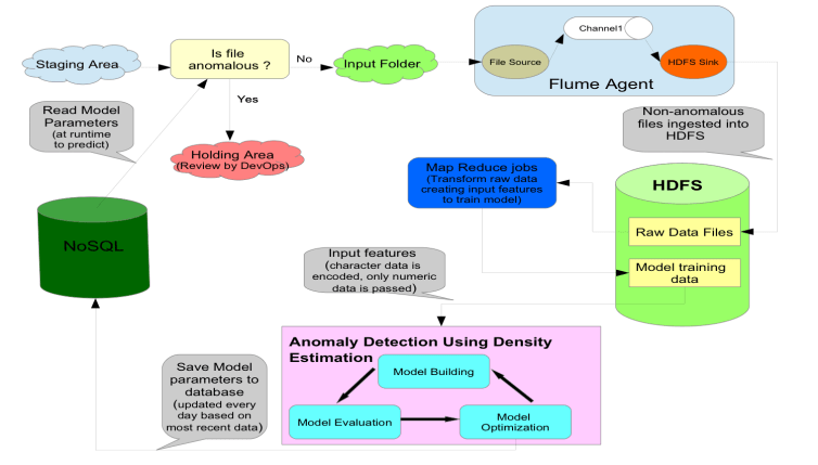
Today, I want to share my thoughts about how we use Unsupervised Machine Learning to detect anomalies in data feeds we receive from our clients as a part of B2B exchange. The aim is to flag anomalies in any external data feeds we receive before they are processed through our system workflows/processes for additional review. This ensures that we are pro-actively reviewing files that could have potential issues and significantly reduces  time our DevOps team is spending in retroactively fixing/troubleshooting issues.

We want to detect in advance if a data feed from an external source (transmission via FTP/SFTP, web service calls, email transmissions etc ) is anomalous in some way. Does it look different from the same type of data we have seen before? Although anomaly detection is mainly an Unsupervised Machine Learning problem, we have to use some aspects Supervised Machine Learning to evaluate our model’s performance. Given some examples of external data feeds that are not anomalous, we want our algorithm to learn from them and tell us if a new feed is anomalous.

Before building a model, we first need to generate for each data feed features that will be used as input for building it. As an example, lets assume that we receive a file (data feed) via SFTP every hour. For each file received every hour, we read its contents  into a set of vectors, where each vector contains data for one specific column. For each vector (that represents data in all rows for a column), we use data type for the column to generate a set of features that would be used as input to train our model. For numeric data type, we calculate mean, range, maximum, minimum for each column and add them as features for building the model. For character data, we calculate unique entries in the vector and store the count as feature for building the model. We use Hadoop to process contents of millions of data feeds as described above and generate datasets that are used as input for building the model.

Let me explain this process in details using an example. Let us assume that we have a file with 3 columns and 4 rows as shown below:

	Col 1 (Numeric data)	Col 2 (Character Data)	Col 3 (Numeric Data)
Row 1	3	Test	100.1
Row 2	4	Test1	100.2
Row 3	2	Testing	100.1
Row 4	4	Test	100.0

On processing the sample file above, we will end up with three vectors as follows

Vector1 – {3, 4, 2, 4}

Vector2 – {“Test”, “Test1”, “Testing”, “Test”}

Vector3 – {100.1, 100.2, 100.1, 100.0}

Based on the process described above, given sample file will generate an output containing 9 features {3.25, 2, 4, 2, 3, 101.1, 0.2, 100.2, 100.0} where

• First 4 elements of feature vector (3.25, 2, 4, 2) are created based on contents of vector representing Col1 (mean, range, maximum and minimum)
• Fifth element of feature vector (3) is created from Col2 (count of unique entries in vector)
• Last 4 elements of feature vector (101.1, 0.2, 100.2, 100.0) are created based on contents of vector representing Col3 (mean, range, maximum and minimum)

All features fed as input to our algorithm contain NUMERIC data only.

Model building using Density Estimation technique:

• Generate one row of n features x_i (where i = 1 to n) for each non-anomalous data feed. We will generate features for all historical non-anomalous data as input for our model.
• Fit parameters  (Mean) and  (Standard Deviation) for all features (i = 0 to n) where    

and   

• Model  from data using the formula 
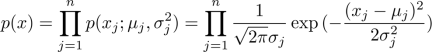
• Given a new data feed, calculate . If the calculated value is less than a given threshold, flag it as anomalous.

 

Evaluating Anomaly Detection:

For Anomaly Detection, we can’t use classification techniques (which are a part of Supervised Machine Learning) because of two reasons:

• Most of available data for learning for our algorithm is non-anomalous files that have been successfully processed.
• It is difficult to predict beforehand with examples what anomalies will look like. Also, future anomalies might look very different from what we have seen till date.

But to evaluate performance of our anomaly detection algorithm, we assume that we have some labelled data of consisting primarily of non-anomalous files with a very small number of anomalous files (less than 0. 1%). We divide the input data sets into three sections:

Training Set (65% of total input datasets): Contains only data from non-anomalous files used to fit the model (calculate  and  ).

Cross Validation Set (25% of total input datasets): Contains very few anomalous files with lots of non-anomalous files to calculate  and flag an anomaly if .

Test Set (remaining 10% of total input datasets): Contains both file types. We use our model to predict if a file is anomalous OR not and compare the predicted value with actual label to determine true positives, true negatives, false positives, false negatives for Test set. These parameters are used to evaluate F-1 score which gives us a single number evaluation score for our algorithm.